Preview Functionality

The FFT Display is currently a preview feature. As such, the content in this page is subject to change based on feedback and roadmap changes. This display is available from ATLAS v11.5.4.230 onwards.

FFT Display#

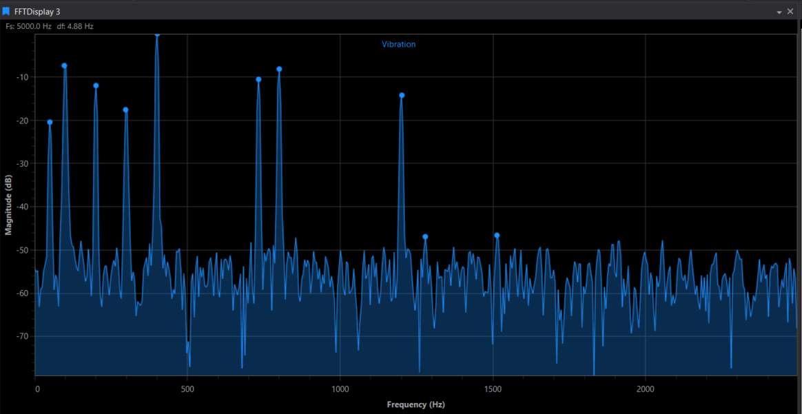
Frequency content of a single parameter. The FFT Display takes the samples in the current session timebase and transforms them into a spectrum — magnitude against frequency — so you can see which frequencies are present in a signal rather than how it varies over time.

FFT Display

When to Use FFT Display#

Vibration analysis: Identify the dominant frequencies in an accelerometer or strain channel.

Rotational orders: Relate spectral peaks to shaft, wheel or engine speeds.

Noise and interference: Spot mains hum, sensor noise or aliasing artefacts in a channel.

Filter checking: Confirm that a filtered signal has actually lost the frequencies you expected.

Enabling the FFT Display#

Note

The FFT Display is off by default. Enable it in Tools > Options > General > Preview Features by ticking Allow FFT display, then restart ATLAS. Until you do, the display does not appear on the toolbar, in the File > New > Display menu, or in the Quick Access Assistant.

Adding an FFT Display#

To add an FFT Display to a page, use one of the following methods:

Display Toolbar: Click the FFT Display button .
Menu: Go to File > New > Display and select FFT Display.
Quick Access Assistant: Press Ctrl + Q twice, then select New FFT Display.

Adding a Parameter#

The FFT Display shows one parameter at a time.

Press P to open the Parameter Browser and select a parameter, or
Drag a parameter onto the display from the Parameter Browser or another display.

Dropping a parameter onto a display that already has one replaces it — you do not need to remove the old parameter first. The spectrum trace, the fill and the peak markers all take the parameter's colour, and the parameter name is shown at the top of the plot.

Display Anatomy#

Header readouts: Fs — the sample rate used for the transform, and df — the frequency resolution (the width of one bin). Both appear at the top left once a spectrum has been computed.
X-Axis: Frequency in Hz, from 0 up to the Nyquist frequency (half the sample rate).
Y-Axis: Magnitude, either linear or in dB.
Spectrum trace: The parameter's spectrum, optionally filled below the curve.
Peak markers: Circular markers on the most prominent peaks.
Status message: Replaces the plot when there is not enough data to transform.

Display Properties#

Press D or right-click > Display Properties to open the property grid.

Category	Property	Default	Description
General	Background Colour	Black	The background colour of the display.
FFT	Logarithmic Scale (dB)	Off	Switches the magnitude axis between linear and dB.
FFT	Window Function	Hann	The window applied before the transform: None, Hann, Hamming or Blackman.
FFT	FFT Size	1024	The maximum number of samples used for the transform.
FFT	Show Fill	On	Shows or hides the shaded area under the spectrum curve.
FFT	Show Peaks	On	Shows or hides the peak markers.

FFT Size#

FFT Size sets the maximum number of samples fed into the transform. It is limited to the range 64 to 16384 and is always snapped to a power of two: entering a larger value rounds up to the next power of two, entering a smaller one rounds down to the previous one. So typing 1000 gives 1024, and typing 900 when the size was 1024 gives 512.

The size you choose trades frequency resolution against the amount of data summarised:

FFT Size	Frequency resolution	Use when
Smaller (64–512)	Coarser	You only need the broad shape of the spectrum.
Default (1024)	Balanced	General-purpose analysis.
Larger (2048–16384)	Finer	You need to separate peaks that are close together in frequency.

If the parameter has fewer samples than the FFT Size, the transform still runs at the next power of two above the sample count, and the remainder is zero-padded.

Window Function#

A window function tapers the ends of the sample block before the transform, which reduces the spectral leakage that would otherwise smear a peak across neighbouring bins.

Window	Character
None	No tapering. Sharpest possible peak, most leakage.
Hann	Good general-purpose compromise between peak width and leakage. Default.
Hamming	Slightly narrower main lobe than Hann, with a higher first side lobe.
Blackman	Widest main lobe, lowest leakage — best for spotting a small peak next to a large one.

Logarithmic Scale#

With Logarithmic Scale (dB) off, the Y-axis shows linear magnitude and is titled Magnitude. With it on, magnitudes are converted to decibels (20 × log₁₀ of the linear magnitude) and the axis is titled Magnitude (dB). The dB view compresses the range, which makes small peaks visible alongside a dominant one.

Note

Switching the scale clears and recomputes the spectrum, so the plot blanks briefly.

Reading the Spectrum#

Hover anywhere on the trace to get a tooltip giving the frequency and the magnitude of the nearest point — the frequency in Hz to two decimal places, and the magnitude to four (in dB when the logarithmic scale is on).

The two header readouts tell you what the spectrum is capable of showing:

Fs is estimated from the timestamps of the samples returned for the session, so it reflects the actual logging rate of the parameter. The highest frequency the plot can show is half of it.
df is the spacing between adjacent points on the frequency axis — the sample rate divided by the transform length. Two components closer together than df cannot be resolved into separate peaks.

In the screenshot above, a parameter logged at 5000 Hz and the default 1024-point transform give a resolution of 4.88 Hz per bin, over a frequency axis reaching 2500 Hz.

Peak Markers#

With Show Peaks on, the display marks the peaks in the spectrum — up to ten of them, chosen by magnitude — with a circular marker. Hover over a marker for its exact frequency and magnitude. Turn Show Peaks off for a cleaner trace when you are only interested in the overall shape.

Action	How
Zoom to a region	Hold the right mouse button and drag a box over the area of interest.
Zoom with the wheel	Scroll up to zoom in, down to zoom out. The zoom centres on the pointer.
Left-drag zoom	Right-click > Zoom Box, then drag once with the left button.
Undo Zoom	Right-click > Undo Zoom. Steps back one zoom level.
Undo All Zooms	Right-click > Undo All Zooms. Returns to the full spectrum.

Both axes auto-range until you zoom. Undoing past the first zoom level restores auto-ranging, so the display resumes fitting the whole spectrum as new data arrives.

Refreshing#

The display recomputes when the data it depends on changes — a new session, a new parameter, or a change to any of the FFT properties. Requests are throttled to five a second, and the spectrum is computed over the whole of the current session timebase rather than a cursor window. Changing or removing the session clears the display.

Troubleshooting#

Symptom	Cause	Fix
The FFT Display is not on the toolbar or in the display menu	The preview feature is not enabled, or ATLAS has not been restarted since enabling it	Tick Allow FFT display in Tools > Options > General > Preview Features and restart ATLAS.
"Insufficient data, please select a wider timeline"	The parameter returned too few samples over the session timebase to compute a transform	Widen the timeline, choose a parameter logged at a higher rate, or open a session with a longer timebase.
The plot is empty and there are no readouts	No parameter has been added, or the session has no data for it	Press `P` and select a parameter, or drag one onto the display.
The peaks you expect are missing or merged	The frequency resolution is too coarse to separate them	Increase FFT Size, or switch Window Function to Blackman if a large peak is masking a small one.
A small peak is invisible next to a large one	Linear magnitude scaling	Turn on Logarithmic Scale (dB).

Quick Reference#

Key	Action
`D`	Display Properties
`P`	Parameter Browser
`Ctrl + Q, Ctrl + Q`	Quick Access Assistant